While administrating the network, it’s important to think about high availability. If one network element goes down, the network can still operate properly after it’s converged. But how about the convergence time? It differs from one protocol to another, and it can take over 30 seconds to detect failure. In such a case, most of the end-users will notice the network outage because of timeouts. So the question is, can we do something to speed up the convergence time? In this article, we will take a look a the OSPF failover scenarios with and without the BFD protocol.
Topology
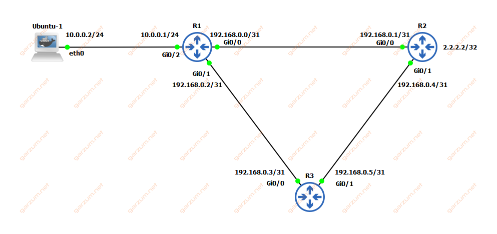
The topology for today’s lab is pretty straightforward. We’ve got a Ubuntu-1 PC, which will be used to test connectivity. Then we have three Cisco routers, R1-R3. On R3 there is configured a loopback interface with a 2.2.2.2 ip address. Between all the routers, there is configured OSPF, which is used to advertise the visible networks and addresses between the routers. All the visible links are the same when it comes to speed and link type.
Scenarios
In normal circumstances, the traffic from Ubuntu-1 to 2.2.2.2 will take the fastest way possible, so in this case packets after reaching R1 will be sent directly to the R2. Only when the failure of the R1-R2 link occurs, the traffic will be sent via the R3 router.
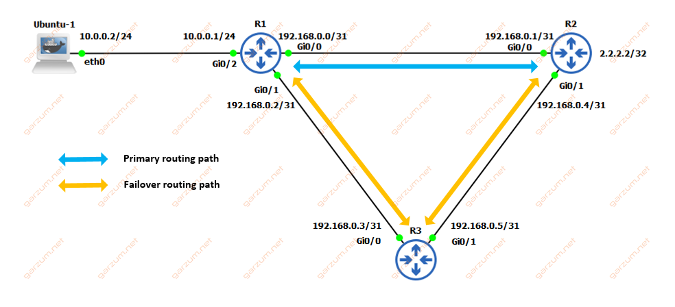
We will simulate the failure of the R1-R2 link with two configurations, with and without BFD configured between those routers. But first of all, let’s take a look at the configuration of each router.
Configuration
R1
On the R1, there is configured a loopback interface with an address of 1.1.1.1. Then we have 3 physical interfaces configuration with descriptions and ipv4 addressing. In the end, there is an OSPF configuration with one network statement, which enables OSPF on all of the interfaces. The configuration of R2 and R3 is very similar.
interface Loopback0
 ip address 1.1.1.1 255.255.255.255
!
interface GigabitEthernet0/0
 description to_R2
 ip address 192.168.0.0 255.255.255.254
 ip ospf network point-to-point
 duplex auto
 speed auto
 media-type rj45
!
interface GigabitEthernet0/1
 description to_R3
 ip address 192.168.0.2 255.255.255.254
 ip ospf network point-to-point
 duplex auto
 speed auto
 media-type rj45
!
interface GigabitEthernet0/2
 description to_Ubuntu-1
 ip address 10.0.0.1 255.255.255.0
 duplex auto
 speed auto
 media-type rj45
!
router ospf 1
 network 0.0.0.0 255.255.255.255 area 0
!
R2
R2
interface Loopback0
 ip address 2.2.2.2 255.255.255.255
!
interface GigabitEthernet0/0
 description to_R1
 ip address 192.168.0.1 255.255.255.254
 ip ospf network point-to-point
 duplex auto
 speed auto
 media-type rj45
!
interface GigabitEthernet0/1
 description to_R3
 ip address 192.168.0.4 255.255.255.254
 ip ospf network point-to-point
 duplex auto
 speed auto
 media-type rj45
!
router ospf 1
 network 0.0.0.0 255.255.255.255 area 0
!
R3
R3
interface Loopback0
 ip address 3.3.3.3 255.255.255.255
!
interface GigabitEthernet0/0
 description to_R1
 ip address 192.168.0.3 255.255.255.254
 ip ospf network point-to-point
 duplex auto
 speed auto
 media-type rj45
!
interface GigabitEthernet0/1
 description to_R2
 ip address 192.168.0.5 255.255.255.254
 ip ospf network point-to-point
 duplex auto
 speed auto
 media-type rj45
!
router ospf 1
 network 0.0.0.0 255.255.255.255 area 0
!
Now, since we know how are the routers configured, let’s check the R1 state.
Pre-check
OSPF neighbors
Let’s start with the OSPF neighbors. R1 should form a neighborship with R2 and R3.
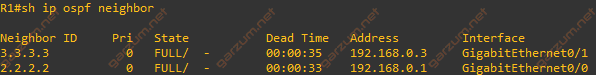
Everything is as expected, we have two neighborships with the FULL state. All the subnets should be advertised across the network.
Routing table
Let’s check the routing table of R1. All the loopback addresses should be visible there.
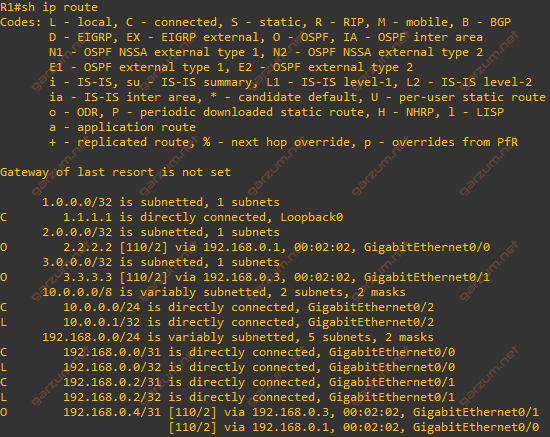
As we can see, the loopbacks of R2 and R3 are visible. We can now check connectivity from the Ubuntu-1 to the R2’s loopback interface.
Connectivity
Connectivity will be tested the easiest way possible – the ping command.
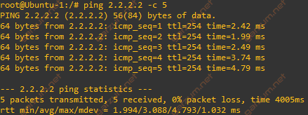
There is a response, so we can assume, that everything works as expected. Let’s jump to the scenarios!
Failover without BFD
First of all, we will simulate the link failure without the BFD. It will give us an overview of how long does it take to recover in such a scenario.
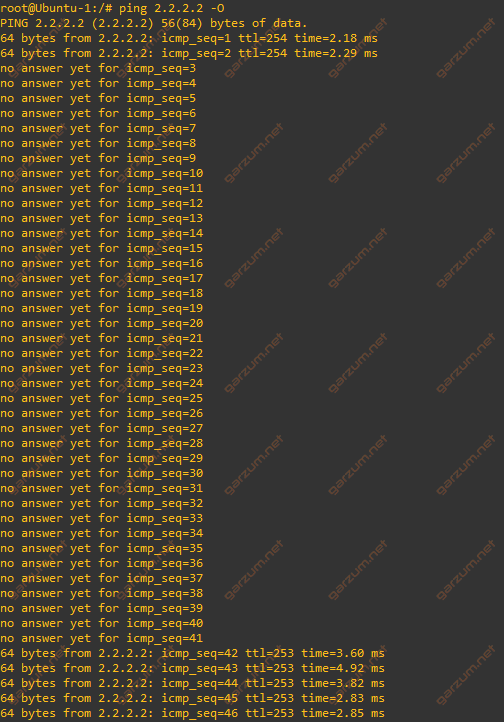
As we can see, after the link failure, there were no answers to the ICMP echo request packets. But after some time, the connectivity was restored.
In summary 39 packets were lost, which gives us about 39 seconds of an outage.
By default, OSPF has configured a dead timer to 40 seconds, and each hello packet is sent every 10 seconds. So if a router doesn’t receive any hello packets within 40 seconds, the neighborship is torn down, and OSPF begins to calculate new best routes for subnets.
If we take a look at the logs on the R1 router, we can see information about the expiration of the dead timer.

Now we can check our neighbors once again, and the neighborship with R2 (2.2.2.2) will disappear.

Since after the link outage, the connectivity to the 2.2.2.2 were restored, let’s take a look at the routing table of R1.

As we can see, the entry for 2.2.2.2 is still in the routing table. Let’s take a closer look.
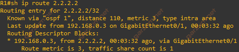
If we take a closer look, we can see that the traffic destined to 2.2.2.2 is going via R3 now.
Failover with BFD
As you can probably guess, when we enhance OSPF with BFD configuration, the converge time can be shortened significantly. In the previous scenario, the OSPF needed about 40 seconds to determine that the neighbor is down. So if we improve the neighborship failure mechanism, the overall converge time should be significantly lower, and that’s where the BFD comes into play! It can be used with various routing protocols, not only with OSPF, but in this article, we will configure it only with the OSPF.
BFD similarly to the OSPF forms neighborships. As you can probably guess, we have to configure in on both routers to form an adjacency. BFD is configurable per interface, so there is no need to implement it on every interface. In this scenario, the BFD neighborship will be formed only on the link between the R1 and R2.
To configure BFD, we need to specify timers. The values can be adjusted by an administrator. It’s important to adjust them properly based on our network infrastructure. BFD sends a huge amount of packets so if the link is used extensively, it can lead to dropped packets, which can cause neighborship to go down. In this case, I’ve chosen the lowest values possible, because it’s a direct connection between the routers, and the link is not used extensively.
BFD timer configuration consists of 3 values:
- interval – how frequently (in milliseconds) BFD packets will be sent to BFD peers
- min_rx – how frequently (in milliseconds) BFD packets will be expected to be received from BFD peers
- multiplier – after missing this number of packets, BFD session is torn down and higher-layer protocols are informed of the failure
The next step is to link BFD with OSPF, we have two options:
- configure it per interface with ip ospf bfd command
- configure it globally in the ospf configuration mode with bfd all-interfaces command
In this case, the BFD is configured per interface. Here’s the configuration of the Gi0/0 interface of R1. The BFD configuration on R2 is similar.
interface GigabitEthernet0/0
 description to_R2
 ip address 192.168.0.0 255.255.255.254
 ip ospf network point-to-point
 ip ospf bfd
 duplex auto
 speed auto
 media-type rj45
 bfd interval 50 min_rx 50 multiplier 3
end
After the configuration of R1 and R2, we should have a formed BFD neighborship between those routers. Let’s check that.
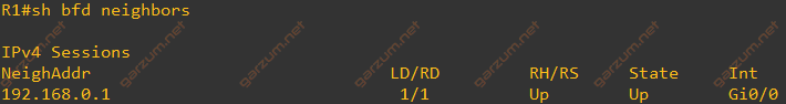
As we can see, there is one neighborship. The address points to the Gi0/0 interface of R2. Adjacency is in the upstate. Let’s check the details.
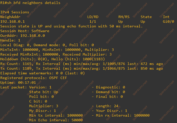
From the command output, we can see, that two protocols are using this neighborship: OSPF and CEF. In case of link failure, the neighborship is torn down, and the protocols that are associated with this neighborship are signaled. In such a scenario, OSPF will tear down its own neighborship too, and that’s exactly what we want. As you can guess from the BFD timers, the time of failure detection should be way faster compared to standard OSPF. Let’s check it!
Once again we will use the ping command to test connectivity.
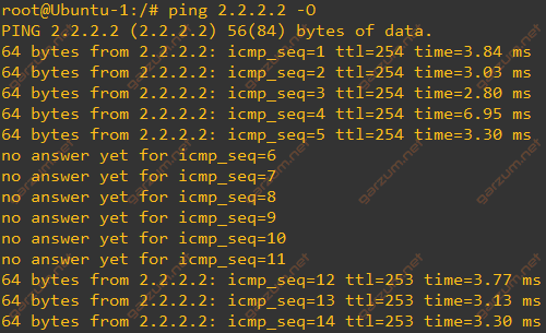
As we can see, this time the outage time is much shorter. In this case, 6 packets are lost, which gives us about 6 seconds of the network outage. The standard OSPF configuration converge time was about 39 seconds, so by configuring BFD alongside OSPF, we speed up the convergence time 6,5 times!
After the link failure detection, there are BFD logs visible on the R1.
